Exam P Practice Problem 110 – likelihood of auto accidents

By Dan Ma on March 4, 2019 | Leave a comment

Problem 110-A

An actuary studied the likelihood of accidents in a one-year period among a large group of insured drivers. The following table gives the results.

Age Group	Percent of Drivers	Probability of 0 Accidents	Probability of 1 Accident
16-20	15%	0.20	0.25
21-30	25%	0.35	0.40
31-50	35%	0.60	0.30
51-70	20%	0.67	0.23
71+	5%	0.50	0.35

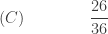
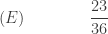
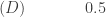
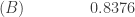
Suppose that a randomly selected insured driver in the studied group had at least 2 accidents in the past year. Calculate the probability that the insured driver is in the age group 21-30.

$\displaystyle \bold ( \bold A \bold ) \ \ \ \ \ \ \ \ \ \ \ \ \bold 0 \bold . \bold 1 \bold 7$

$\displaystyle \bold ( \bold B \bold ) \ \ \ \ \ \ \ \ \ \ \ \ \bold 0 \bold . \bold 2 \bold 4$

$\displaystyle \bold ( \bold C \bold ) \ \ \ \ \ \ \ \ \ \ \ \ \bold 0 \bold . \bold 3 \bold 0$

$\displaystyle \bold ( \bold D \bold ) \ \ \ \ \ \ \ \ \ \ \ \ \bold 0 \bold . \bold 4 \bold 0$

$\displaystyle \bold ( \bold E \bold ) \ \ \ \ \ \ \ \ \ \ \ \ \bold 0 \bold . \bold 4 \bold 5$

$\text{ }$

Problem 110-B

An auto insurance company performed a study on the frequency of accidents of its insured drivers in a one-year period. The following table gives the results of the study.

Age Group	Percent of Drivers	Probability of At Least 1 Accident
16-20	10%	0.30
21-40	20%	0.20
41-65	35%	0.10
66+	35%	0.12

A randomly selected insured driver from the study was found to have no accidents in the one-year period.

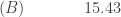
Calculate the probability that the insured driver is from the age group 16-20.

$\displaystyle \bold ( \bold A \bold ) \ \ \ \ \ \ \ \ \ \ \ \ \bold 0 \bold . \bold 0 \bold 8$

$\displaystyle \bold ( \bold B \bold ) \ \ \ \ \ \ \ \ \ \ \ \ \bold 0 \bold . \bold 1 \bold 2$

$\displaystyle \bold ( \bold C \bold ) \ \ \ \ \ \ \ \ \ \ \ \ \bold 0 \bold . \bold 1 \bold 5$

$\displaystyle \bold ( \bold D \bold ) \ \ \ \ \ \ \ \ \ \ \ \ \bold 0 \bold . \bold 1 \bold 9$

$\displaystyle \bold ( \bold E \bold ) \ \ \ \ \ \ \ \ \ \ \ \ \bold 0 \bold . \bold 2 \bold 0$

$\text{ }$

Answers

this page

exam P practice problem

probability exam P

actuarial exam

actuarial practice problem

math

Daniel Ma

mathematics

dan ma actuarial science

daniel ma actuarial science

Daniel Ma actuarial

$\copyright$ 2019 – Dan Ma

Posted in: Insurance and Risk Management, Practice Problems, Uncategorized | Tagged: Bayes' Theorem, The law of total probability

Exam P Practice Problem 109 – counting insurance payments

By Dan Ma on February 25, 2019 | Leave a comment

Problem 109-A

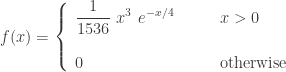
Amounts of damages due to auto collision accidents follow a probability distribution whose density function is given by the following.

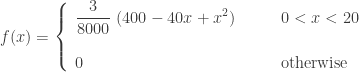
$\displaystyle f(x) = \left\{ \begin{array}{ll} \displaystyle \frac{3}{8000} \ (400-40x+x^2) &\ \ \ \ \ \ 0 < x < 20 \\ \text{ } & \text{ } \\ \displaystyle 0 &\ \ \ \ \ \ \text{otherwise} \\ \end{array} \right.$

When occurred, the collision damages are reimbursed by an insurance coverage subject to a deductible of 4.

Fifteen unrelated auto collision accidents have been reported. Determine the probability that exactly nine or ten of the accidents will be reimbursed by the insurance coverage.

$\displaystyle \bold ( \bold A \bold ) \ \ \ \ \ \ \ \ \ \ \ \ \bold 0 \bold . \bold 1 \bold 4 \bold 2$

$\displaystyle \bold ( \bold B \bold ) \ \ \ \ \ \ \ \ \ \ \ \ \bold 0 \bold . \bold 1 \bold 6 \bold 3$

$\displaystyle \bold ( \bold C \bold ) \ \ \ \ \ \ \ \ \ \ \ \ \bold 0 \bold . \bold 2 \bold 2 \bold 2$

$\displaystyle \bold ( \bold D \bold ) \ \ \ \ \ \ \ \ \ \ \ \ \bold 0 \bold . \bold 2 \bold 6 \bold 6$

$\displaystyle \bold ( \bold E \bold ) \ \ \ \ \ \ \ \ \ \ \ \ \bold 0 \bold . \bold 2 \bold 8 \bold 9$

$\text{ }$

Problem 109-B

Amounts of damages due to auto collision accidents follow a probability distribution whose density function is given by the following.

$\displaystyle f(x) = \left\{ \begin{array}{ll} \displaystyle \frac{3}{4000} \ (400-80x+4 x^2) &\ \ \ \ \ \ 0 < x < 10 \\ \text{ } & \text{ } \\ \displaystyle 0 &\ \ \ \ \ \ \text{otherwise} \\ \end{array} \right.$

When occurred, the damages are reimbursed by an insurance coverage subject to a deductible of 2.

Twelve unrelated auto collision accidents have been reported. Determine the probability that exactly six or seven of the accidents will not be reimbursed by the insurance coverage.

$\displaystyle \bold ( \bold A \bold ) \ \ \ \ \ \ \ \ \ \ \ \ \bold 0 \bold . \bold 1 \bold 8 \bold 4$

$\displaystyle \bold ( \bold B \bold ) \ \ \ \ \ \ \ \ \ \ \ \ \bold 0 \bold . \bold 2 \bold 2 \bold 5$

$\displaystyle \bold ( \bold C \bold ) \ \ \ \ \ \ \ \ \ \ \ \ \bold 0 \bold . \bold 4 \bold 0 \bold 8$

$\displaystyle \bold ( \bold D \bold ) \ \ \ \ \ \ \ \ \ \ \ \ \bold 0 \bold . \bold 4 \bold 2 \bold 7$

$\displaystyle \bold ( \bold E \bold ) \ \ \ \ \ \ \ \ \ \ \ \ \bold 0 \bold . \bold 4 \bold 5 \bold 0$

$\text{ }$

Answers

this page

exam P practice problem

probability exam P

actuarial exam

actuarial practice problem

math

Daniel Ma

mathematics

dan ma actuarial science

daniel ma actuarial science

Daniel Ma actuarial

$\copyright$ 2019 – Dan Ma

Posted in: Insurance and Risk Management, Practice Problems | Tagged: Binomial distribution, deductible

Exam P Practice Problem 108 – random selection of balls

By Dan Ma on February 3, 2019 | Leave a comment

Both 108-A and 108-B use the following information.

Bowl One contains 1 blue ball and 4 orange balls. Bowl Two contains 3 blue balls and 2 orange balls. A bowl is chosen at random. Balls are randomly chosen one at a time from the chosen bowl, with each chosen ball returning to the bowl.

Problem 108-A

What is the probability that four of the first six selections are blue ball?

$\displaystyle \bold ( \bold A \bold ) \ \ \ \ \ \ \ \ \ \ \ \ \frac{\bold 4 \bold 8 \bold 6}{\bold 3 \bold 1 \bold 2 \bold 5}$

$\displaystyle \bold ( \bold B \bold ) \ \ \ \ \ \ \ \ \ \ \ \ \frac{\bold 1 \bold 0 \bold2}{\bold 6 \bold 2 \bold 5}$

$\displaystyle \bold ( \bold C \bold ) \ \ \ \ \ \ \ \ \ \ \ \ \frac{\bold 3 \bold 4}{\bold 2 \bold 0 \bold 5}$

$\displaystyle \bold ( \bold D \bold ) \ \ \ \ \ \ \ \ \ \ \ \ \frac{\bold 2 \bold 1}{\bold 1 \bold 2 \bold 5}$

$\displaystyle \bold ( \bold E \bold ) \ \ \ \ \ \ \ \ \ \ \ \ \frac{\bold 1 \bold 0 \bold 2 \bold 0}{\bold 3 \bold 1 \bold 2 \bold 5}$

$\text{ }$

Problem 108-B

If four of the first six selections are blue balls, what is the probability that the balls are selected from Bowl One?

$\displaystyle \bold ( \bold A \bold ) \ \ \ \ \ \ \ \ \ \ \ \ \frac{\bold 9}{\bold 2 \bold 5 \bold 5}$

$\displaystyle \bold ( \bold B \bold ) \ \ \ \ \ \ \ \ \ \ \ \ \frac{\bold 2}{\bold 4 \bold 3}$

$\displaystyle \bold ( \bold C \bold ) \ \ \ \ \ \ \ \ \ \ \ \ \frac{\bold 4}{\bold 8 \bold 5}$

$\displaystyle \bold ( \bold D \bold ) \ \ \ \ \ \ \ \ \ \ \ \ \frac{\bold 1 \bold 5}{\bold 2 \bold 5 \bold 5}$

$\displaystyle \bold ( \bold E \bold ) \ \ \ \ \ \ \ \ \ \ \ \ \frac{\bold 1}{\bold 2}$

$\text{ }$

Answers

this page

probability exam P

actuarial exam

math

Daniel Ma

mathematics

dan ma actuarial science

daniel ma actuarial science

Daniel Ma actuarial

dan ma statistical actuarial

daniel ma statistical actuarial

$\copyright$ 2019 – Dan Ma

Posted in: Practice Problems | Tagged: Bayes' Theorem, Binomial distribution, Mixed Distribution

Exam P Practice Problem 107 – wait time at a busy restaurant

By Dan Ma on January 22, 2019 | Leave a comment

Both 107-A and 107-B use the following probability density function.

$\displaystyle f(x) = \left\{ \begin{array}{ll} \displaystyle \frac{1}{450} \ (30-x) &\ \ \ \ \ \ 0 < x < 30 \\ \text{ } & \text{ } \\ \displaystyle 0 &\ \ \ \ \ \ \text{otherwise} \\ \end{array} \right.$

Problem 107-A

The wait time (in minutes) for a table at a busy restaurant on the weekend is distributed according to the density function $f(x)$ given above.

A customer plans to dine in this restaurant on two different weekends.

Determine the expected value of the longest wait of these two visits to the restaurant.

$\displaystyle \bold ( \bold A \bold ) \ \ \ \ \ \ \ \ \ \ \ \ \bold 1 \bold 0 \bold . \bold 0$

$\displaystyle \bold ( \bold B \bold ) \ \ \ \ \ \ \ \ \ \ \ \ \bold 1 \bold 1 \bold . \bold 0$

$\displaystyle \bold ( \bold C \bold ) \ \ \ \ \ \ \ \ \ \ \ \ \bold 1 \bold 2 \bold . \bold 8$

$\displaystyle \bold ( \bold D \bold ) \ \ \ \ \ \ \ \ \ \ \ \ \bold 1 \bold 3 \bold . \bold 5$

$\displaystyle \bold ( \bold E \bold ) \ \ \ \ \ \ \ \ \ \ \ \ \bold 1 \bold 4 \bold . \bold 0$

$\text{ }$

Problem 107-B

The wait time (in minutes) for a table at a busy restaurant on the weekend is distributed according to the density function $f(x)$ given above.

A customer plans to dine in this restaurant on two different weekends.

Determine the expected value of the shortest wait of these two visits to the restaurant.

$\displaystyle \bold ( \bold A \bold ) \ \ \ \ \ \ \ \ \ \ \ \ \bold 4 \bold . \bold 5$

$\displaystyle \bold ( \bold B \bold ) \ \ \ \ \ \ \ \ \ \ \ \ \bold 6 \bold . \bold 0$

$\displaystyle \bold ( \bold C \bold ) \ \ \ \ \ \ \ \ \ \ \ \ \bold 7 \bold . \bold 0$

$\displaystyle \bold ( \bold D \bold ) \ \ \ \ \ \ \ \ \ \ \ \ \bold 8 \bold . \bold 6$

$\displaystyle \bold ( \bold E \bold ) \ \ \ \ \ \ \ \ \ \ \ \ \bold 1 \bold 0 \bold . \bold 0$

$\text{ }$

Answers

this page

probability exam P

actuarial exam

math

Daniel Ma

mathematics

dan ma actuarial science

daniel ma actuarial science

Daniel Ma actuarial

dan ma statistical actuarial

daniel ma statistical actuarial

$\copyright$ 2019 – Dan Ma

Posted in: Practice Problems | Tagged: Order Statistics

Exam P Practice Problem 106 – average height of students

By Dan Ma on January 12, 2019 | Leave a comment

Problem 106-A

Heights of male students in a large university follow a normal distribution with mean 69 inches and standard deviation 2.8 inches.

Four male students from this university are randomly selected.

Determine the probability that the average height of the selected students is between 5 feet 7 inches and 5 feet 11 inches.

Note that one feet = 12 inches.

$\displaystyle \bold ( \bold A \bold ) \ \ \ \ \ \ \ \ \ \ \ \ \bold 0 \bold . \bold 1 \bold 1 \bold 0 \bold 4$

$\displaystyle \bold ( \bold B \bold ) \ \ \ \ \ \ \ \ \ \ \ \ \bold 0 \bold . \bold 5 \bold 2 \bold 2 \bold 2$

$\displaystyle \bold ( \bold C \bold ) \ \ \ \ \ \ \ \ \ \ \ \ \bold 0 \bold . \bold 8 \bold 4 \bold 7 \bold 2$

$\displaystyle \bold ( \bold D \bold ) \ \ \ \ \ \ \ \ \ \ \ \ \bold 0 \bold . \bold 8 \bold 8 \bold 9 \bold 6$

$\displaystyle \bold ( \bold E \bold ) \ \ \ \ \ \ \ \ \ \ \ \ \bold 0 \bold . \bold 9 \bold 0 \bold 7 \bold 5$

The answers are based on this normal table from SOA.

$\text{ }$

Problem 106-B

Heights of female students in a large university follow a normal distribution with mean 65 inches and standard deviation 2.2 inches.

Sixteen female students are randomly selected.

Determine the probability that the average height of the selected students is greater than 5 feet 6 inches.

Note that one feet = 12 inches.

$\displaystyle \bold ( \bold A \bold ) \ \ \ \ \ \ \ \ \ \ \ \ \bold 0 \bold . \bold 0 \bold 3 \bold 4 \bold 4$

$\displaystyle \bold ( \bold B \bold ) \ \ \ \ \ \ \ \ \ \ \ \ \bold 0 \bold . \bold 1 \bold 7 \bold 8 \bold 2$

$\displaystyle \bold ( \bold C \bold ) \ \ \ \ \ \ \ \ \ \ \ \ \bold 0 \bold . \bold 3 \bold 2 \bold 6 \bold 4$

$\displaystyle \bold ( \bold D \bold ) \ \ \ \ \ \ \ \ \ \ \ \ \bold 0 \bold . \bold 4 \bold 5 \bold 7 \bold 2$

$\displaystyle \bold ( \bold E \bold ) \ \ \ \ \ \ \ \ \ \ \ \ \bold 0 \bold . \bold 6 \bold 7 \bold 3 \bold 6$

The answers are based on this normal table from SOA.

$\text{ }$

Answers

this page

probability exam P

actuarial exam

math

Daniel Ma

mathematics

dan ma actuarial science

daniel ma actuarial science

Daniel Ma actuarial

$\copyright$ 2019 – Dan Ma

Posted in: Normal Distribution, Practice Problems | Tagged: Normal Distribution

Exam P Practice Problem 105 – testing electronic devices

By Dan Ma on January 9, 2019 | Leave a comment

Problem 105-A

The length of operation (in years) for an electronic device follows an exponential distribution with mean 4. Ten such devices are being observed for one year for a quality control study.

The lengths of operation for these devices are independent.

Determine the probability that no more than three of the devices stop working before the end of the study.

$\displaystyle \bold ( \bold A \bold ) \ \ \ \ \ \ \ \ \ \ \ \ \bold 0 \bold . \bold 2 \bold 2 \bold 5 \bold 7$

$\displaystyle \bold ( \bold B \bold ) \ \ \ \ \ \ \ \ \ \ \ \ \bold 0 \bold . \bold 6 \bold 1 \bold 3 \bold 2$

$\displaystyle \bold ( \bold C \bold ) \ \ \ \ \ \ \ \ \ \ \ \ \bold 0 \bold . \bold 7 \bold 5 \bold 6 \bold 8$

$\displaystyle \bold ( \bold D \bold ) \ \ \ \ \ \ \ \ \ \ \ \ \bold 0 \bold . \bold 8 \bold 3 \bold 8 \bold 9$

$\displaystyle \bold ( \bold E \bold ) \ \ \ \ \ \ \ \ \ \ \ \ \bold 0 \bold . \bold 8 \bold 5 \bold 6 \bold 0$

$\text{ }$

Problem 105-B

Twelve patients are randomly selected from a population of patients with history of heart disease to be tracked in a health study. The study begins with an initial assessment of health status. The participants are instructed to return for a follow up visit one year after the initial assessment.

For these patients, the time (in years) from the initial assessment to the next heart attack has an exponential distribution with mean 6.25 years. The times to the next heart attack for these patients are independent.

Determine the probability that ten or more patients experience no heart attack prior to the one-year follow up visit.

$\displaystyle \bold ( \bold A \bold ) \ \ \ \ \ \ \ \ \ \ \ \ \bold 0 \bold . \bold 2 \bold 9 \bold 1 \bold 3$

$\displaystyle \bold ( \bold B \bold ) \ \ \ \ \ \ \ \ \ \ \ \ \bold 0 \bold . \bold 4 \bold 5 \bold 1 \bold 9$

$\displaystyle \bold ( \bold C \bold ) \ \ \ \ \ \ \ \ \ \ \ \ \bold 0 \bold . \bold 5 \bold 4 \bold 8 \bold 1$

$\displaystyle \bold ( \bold D \bold ) \ \ \ \ \ \ \ \ \ \ \ \ \bold 0 \bold . \bold 6 \bold 4 \bold 5 \bold 5$

$\displaystyle \bold ( \bold E \bold ) \ \ \ \ \ \ \ \ \ \ \ \ \bold 0 \bold . \bold 7 \bold 4 \bold 3 \bold 2$

$\text{ }$

Answers

this page

probability exam P

actuarial exam

math

Daniel Ma

mathematics

dan ma actuarial science

daniel ma actuarial science

Daniel Ma actuarial

$\copyright$ 2019 – Dan Ma

Posted in: Exponential distribution | Tagged: Bernoulli distribution, Binomial distribution, Exponential distribution

Exam P Practice Problem 104 – two random insurance losses

By Dan Ma on December 16, 2018 | 1 Comment

Problem 104-A

Two random losses $X$ and $Y$ are jointly modeled by the following density function:

$\displaystyle f(x,y)=\frac{1}{32} \ (4-x) \ (4-y) \ \ \ \ \ \ 0<x<4, \ 0<y<x$

Suppose that both of these losses had occurred. Given that $X$ is exactly 2, what is the probability that $Y$ is less than 1?

$\displaystyle (A) \ \ \ \ \ \ \ \ \ \ \ \ \frac{7}{24}$

$\displaystyle (B) \ \ \ \ \ \ \ \ \ \ \ \ \frac{11}{24}$

$\displaystyle (C) \ \ \ \ \ \ \ \ \ \ \ \ \frac{12}{24}$

$\displaystyle (D) \ \ \ \ \ \ \ \ \ \ \ \ \frac{13}{24}$

$\displaystyle (E) \ \ \ \ \ \ \ \ \ \ \ \ \frac{14}{24}$

$\text{ }$

Problem 104-B

Two random losses $X$ and $Y$ are jointly modeled by the following density function:

$\displaystyle f(x,y)=\frac{1}{96} \ (x+2y) \ \ \ \ \ \ 0<x<4, \ 0<y<4$

Suppose that both of these losses had occurred. Determine the probability that $Y$ exceeds 2 given that the loss $X$ is known to be 2.

$\displaystyle (A) \ \ \ \ \ \ \ \ \ \ \ \ \frac{13}{36}$

$\displaystyle (B) \ \ \ \ \ \ \ \ \ \ \ \ \frac{24}{36}$

$\displaystyle (C) \ \ \ \ \ \ \ \ \ \ \ \ \frac{26}{36}$

$\displaystyle (D) \ \ \ \ \ \ \ \ \ \ \ \ \frac{28}{36}$

$\displaystyle (E) \ \ \ \ \ \ \ \ \ \ \ \ \frac{29}{36}$

$\text{ }$

Answers

this page

probability exam P

actuarial exam

math

Daniel Ma

mathematics

dan ma actuarial science

Daniel Ma actuarial

Posted in: Practice Problems | Tagged: Actuarial Exam, CAS Exam 1, Exam P, Exam P Practice Problems, Joint Distribution, SOA Exam P

Exam P Practice Problem 103 – randomly selected auto collision claims

By Dan Ma on April 9, 2018 | Leave a comment

Problem 103-A

The size of an auto collision claim follows a distribution that has density function 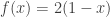$f(x)=2(1-x)$ where $0<x<1$ .

Two randomly selected claims are examined. Compute the probability that one claim is at least twice as large as the other.

$\text{ }$

$\displaystyle (A) \ \ \ \ \ \ \ \ \ \ \ \ \frac{10}{36}$

$\displaystyle (B) \ \ \ \ \ \ \ \ \ \ \ \ \frac{15}{36}$

$\displaystyle (C) \ \ \ \ \ \ \ \ \ \ \ \ \frac{20}{36}$

$\displaystyle (D) \ \ \ \ \ \ \ \ \ \ \ \ \frac{21}{36}$

$\displaystyle (E) \ \ \ \ \ \ \ \ \ \ \ \ \frac{23}{36}$

$\text{ }$

Problem 103-B

Auto collision claims follow an exponential distribution with mean 2.

For two randomly selected auto collision claims, compute the probability that the larger claim is more than four times the size of the smaller claims.

$\text{ }$

$\displaystyle (A) \ \ \ \ \ \ \ \ \ \ \ 0.2$

$\displaystyle (B) \ \ \ \ \ \ \ \ \ \ \ 0.3$

$\displaystyle (C) \ \ \ \ \ \ \ \ \ \ \ 0.4$

$\displaystyle (D) \ \ \ \ \ \ \ \ \ \ \ 0.5$

$\displaystyle (E) \ \ \ \ \ \ \ \ \ \ \ 0.6$

$\text{ }$

Answers can be found in this page.

probability exam P

actuarial exam

math

Daniel Ma

mathematics

dan ma actuarial science

Daniel Ma actuarial

Posted in: Practice Problems | Tagged: Actuarial Exam, CAS Exam 1, Exam P, Exam P Practice Problems, SOA Exam P

Exam P Practice Problem 102 – estimating claim costs

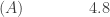
By Dan Ma on January 15, 2018 | Leave a comment

Problem 102-A

Insurance claims modeled by a distribution with the following cumulative distribution function.

$\displaystyle F(x) = \left\{ \begin{array}{ll} \displaystyle 0 &\ \ \ \ \ \ x \le 0 \\ \text{ } & \text{ } \\ \displaystyle \frac{1}{1536} \ x^4 &\ \ \ \ \ \ 0 < x \le 4 \\ \text{ } & \text{ } \\ \displaystyle 1-\frac{2}{3} x+\frac{1}{8} x^2- \frac{1}{1536} \ x^4 &\ \ \ \ \ \ 4 < x \le 8 \\ \text{ } & \text{ } \\ \displaystyle 1 &\ \ \ \ \ \ x > 8 \\ \end{array} \right.$

The insurance company is performing a study on all claims that exceed 3. Determine the mean of all claims being studied.

$\text{ }$

$\displaystyle (A) \ \ \ \ \ \ \ \ \ \ \ \ 4.8$

$\displaystyle (B) \ \ \ \ \ \ \ \ \ \ \ \ 4.9$

$\displaystyle (C) \ \ \ \ \ \ \ \ \ \ \ \ 5.0$

$\displaystyle (D) \ \ \ \ \ \ \ \ \ \ \ \ 5.1$

$\displaystyle (E) \ \ \ \ \ \ \ \ \ \ \ \ 5.2$

$\text{ }$

Problem 102-B

Insurance claims modeled by a distribution with the following cumulative distribution function.

$\displaystyle F(x) = \left\{ \begin{array}{ll} \displaystyle 0 &\ \ \ \ \ \ x \le 0 \\ \text{ } & \text{ } \\ \displaystyle \frac{1}{50} \ x^2 &\ \ \ \ \ \ 0 < x \le 5 \\ \text{ } & \text{ } \\ \displaystyle -\frac{1}{50} x^2+\frac{2}{5} x- 1 &\ \ \ \ \ \ 5 < x \le 10 \\ \text{ } & \text{ } \\ \displaystyle 1 &\ \ \ \ \ \ x > 10 \\ \end{array} \right.$

The insurance company is performing a study on all claims that exceed 4. Determine the mean of all claims being studied.

$\text{ }$

$\displaystyle (A) \ \ \ \ \ \ \ \ \ \ \ 5.9$

$\displaystyle (B) \ \ \ \ \ \ \ \ \ \ \ 6.0$

$\displaystyle (C) \ \ \ \ \ \ \ \ \ \ \ 6.1$

$\displaystyle (D) \ \ \ \ \ \ \ \ \ \ \ 6.2$

$\displaystyle (E) \ \ \ \ \ \ \ \ \ \ \ 6.3$

$\text{ }$

Answers can be found in this page.

probability exam P

actuarial exam

math

Daniel Ma

mathematics

dan ma actuarial science

Daniel Ma actuarial

Posted in: Insurance and Risk Management | Tagged: CAS Exam 1, Exam P, Exam P Practice Problems, Expected Value, Insurance and risk management, SOA Exam P

Exam P Practice Problem 101 – auto collision claims

By Dan Ma on December 17, 2017 | Leave a comment

Problem 101-A

The amount paid on an auto collision claim by an insurance company follows a distribution with the following density function.

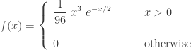
$\displaystyle f(x) = \left\{ \begin{array}{ll} \displaystyle \frac{1}{96} \ x^3 \ e^{-x/2} &\ \ \ \ \ \ x > 0 \\ \text{ } & \text{ } \\ \displaystyle 0 &\ \ \ \ \ \ \text{otherwise} \\ \end{array} \right.$

The insurance company paid 64 claims in a certain month. Determine the approximate probability that the average amount paid is between 7.36 and 8.84.

$\text{ }$

$\displaystyle (A) \ \ \ \ \ \ \ \ \ \ \ \ 0.8320$

$\displaystyle (B) \ \ \ \ \ \ \ \ \ \ \ \ 0.8376$

$\displaystyle (C) \ \ \ \ \ \ \ \ \ \ \ \ 0.8435$

$\displaystyle (D) \ \ \ \ \ \ \ \ \ \ \ \ 0.8532$

$\displaystyle (E) \ \ \ \ \ \ \ \ \ \ \ \ 0.8692$

$\text{ }$

Problem 101-B

The amount paid on an auto collision claim by an insurance company follows a distribution with the following density function.

$\displaystyle f(x) = \left\{ \begin{array}{ll} \displaystyle \frac{1}{1536} \ x^3 \ e^{-x/4} &\ \ \ \ \ \ x > 0 \\ \text{ } & \text{ } \\ \displaystyle 0 &\ \ \ \ \ \ \text{otherwise} \\ \end{array} \right.$

The insurance company paid 36 claims in a certain month. Determine the approximate 25th percentile for the average claims paid in that month.

$\text{ }$

$\displaystyle (A) \ \ \ \ \ \ \ \ \ \ \ 15.11$

$\displaystyle (B) \ \ \ \ \ \ \ \ \ \ \ 15.43$

$\displaystyle (C) \ \ \ \ \ \ \ \ \ \ \ 15.75$

$\displaystyle (D) \ \ \ \ \ \ \ \ \ \ \ 16.25$

$\displaystyle (E) \ \ \ \ \ \ \ \ \ \ \ 16.78$

$\text{ }$

Answers can be found in this page.

probability exam P

actuarial exam

math

Daniel Ma

mathematics

dan ma actuarial science

Daniel Ma actuarial

Posted in: Practice Problems | Tagged: Actuarial Exam, CAS Exam 1, Central Limit Theorem, Exam P, Exam P Practice Problems, Gamma distribution, Normal Distribution, SOA Exam P

SOA Exam P / CAS Exam 1

Exam P Practice Problem 110 – likelihood of auto accidents

Exam P Practice Problem 109 – counting insurance payments

Exam P Practice Problem 108 – random selection of balls

Exam P Practice Problem 107 – wait time at a busy restaurant

Exam P Practice Problem 106 – average height of students

Exam P Practice Problem 105 – testing electronic devices

Exam P Practice Problem 104 – two random insurance losses

Exam P Practice Problem 103 – randomly selected auto collision claims

Exam P Practice Problem 102 – estimating claim costs

Exam P Practice Problem 101 – auto collision claims

Pages

Archives

Email Subscription

Categories

Recent Posts