The method of convolution is a great technique for finding the probability density function (pdf) of the sum of two independent random variables. We state the convolution formula in the continuous case as well as discussing the thought process. Some examples are provided to demonstrate the technique and are followed by an exercise.
The Convolution Formula (Continuous Case)
Let  and
and  be independent continuous random variables with pdfs
  and
and  , respectively. Let
  . Then the following is the pdf of
  .
.

Let’s look at the thought process behind the formula. Since and are independent, the joint pdf of and is  . The pdf of is simply the sum of the “joint density” at the points of the line
  . In Figure 1 below, every point at the line is of the form
  . The joint density at each such point is
  . Summing the values of these joint density produces the probability density function of .

Setting the limits of the integral depends on knowing the range of possible values of  or
or  for a given line . If and can only take on positive values, then for a given line , both or can range from
  to
to  (see Example 1 below).
Example 1
Let and be independent exponentially distributed variables with common density  where
where  . Then the following is the pdf of .

The above pdf indicates that the independent sum of two identically distributed exponential variables has a Gamma distribution with parameters  and
and  .
.
Example 2
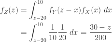
Let and be independent uniformly distributed variables,  and
and  , respectively. The pdf of is:
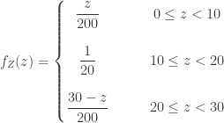
The convolution formula is applied three times. For the first case, the line  ranges in
  . For each such line, we have
  . Figure 2 below is a representative diagram.


For the second case, the line ranges in  . For each such line, ranges from to
  . Figure 3 below is a representative diagram.


For the third case, the line ranges in  . Figure 4 below is a representative diagram.

The following is the graph of the pdf of .

Exercise
Suppose that is an exponentially distributed variable with pdf and has the uniform distribution  . Find the pdf of the independent sum .

